Per's Public Data Repository
Statistics - Probabillity Basics
Joint and Conditional Probabilities, Bayes Theorem, CLT and LTP
Table of contents for notes on probability basics:
Joint Probability
The probability of two events occurring simultaneously. The events should be independent of each other, meaning that the occurrence of one event does not affect the probability of the other event occurring.
Mathematically, the joint probability of two events A and B is denoted as \(P(A ∩ B)\) and is defined as: \(P(A \cap B) = P(A) \cdot P(B)\)
A venn diagram is a useful way to visualize joint probability.
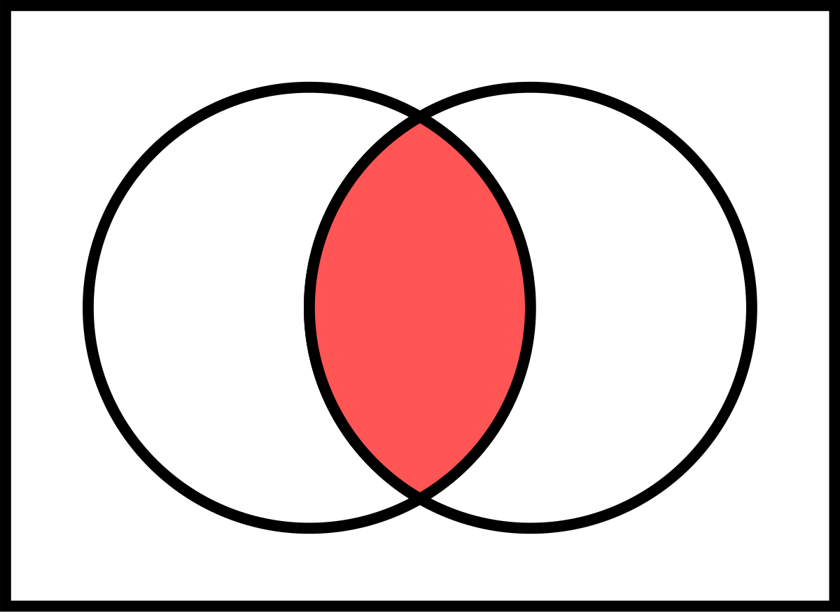
(Image from Wikipedia)
Some examples of joint probability:
- The probability of rolling a 2 and a 3 on a pair of dice is \(\frac{1}{36}\).
- The probability of drawing a 3 of hearts and a 4 of spades from a deck of cards is \(\frac{1}{52} \cdot \frac{1}{51}\).
- The probability of a coin landing on heads and a die landing on 6 is \(\frac{1}{2} \cdot \frac{1}{6}\).
When applied to NLP, joint probability would represent the chances of a sequence of words occurring together. Take for example the sentence “I love you”. The joint probability of the words “I”, “love”, and “you” occurring together would be the ovefrall probability of the sentence occurring in your dataset.
A simple set-up here is to assign a word’s probability of occuring as the number of times it shows up in a corpus divided by the total number of words in the corpus. For example, if the word “I” occurs 100 times in a corpus of 1000 words, then its probability of occurring is \(\frac{100}{1000} = 0.1\). Then assume “love” occurs only 30 times, and “you” occurs 70 times. The joint probability of the sentence “I love you” showing up in the corpus is then \(0.1 \cdot 0.03 \cdot 0.07 = 0.00021\).
This is a very simple example, and could serve as a baseline for more complex models. For example, we could use a Markov model to predict the probability of a word occurring given the previous word. This would be a conditional probability, which we’ll discuss next.
Conditional Probability
The probability of an event occurring given that another event has already occurred. Again, the events could dependent or independent of each other. Unlike joint probability, the events are not necessarily occurring simultaneously.
Mathematically, the conditional probability of two events A and B is denoted as \(P(A \mid B)\) and is defined as:
\[P(A \mid B) = \frac{P(A \cap B)}{P(B)}\]A nice way to visualize conditional probability is with a tree diagram.

(Image from Wikipedia)
Some examples of conditional probability:
- The probability of rolling a 3 on a die given that the number is odd is \(\frac{1}{3}\).
- The probability of drawing a 4 of spades from a deck of cards given that the card is a spade is \(\frac{1}{13}\).
- The probability of a coin landing on heads given that a die lands on 6 is \(\frac{1}{2}\).
When applied to NLP, conditional probability would represent the chances of a word occurring given the previous word. Take for example the sentence “I love you”. The conditional probability of the word “love” occurring given that the word “I” has already occurred would be the probability of the word “love” occurring in the corpus after the word “I” has already occurred. One way to find determine probability of word-pair occurances is to break the corpus into two-word tuples.
For example, the sentence “I love you” would be broken into the tuples “I love” and “love you”. Then the conditional probability of the word “love” occurring given that the word “I” has already occurred would be the number of times the tuple “I love” occurs in the corpus divided by the number of times the word “I” occurs in the corpus. So, following our example from above, if the word “I” occurs 100 times in a corpus of 1000 words, and the tuple “I love” occurs 20 times, then the conditional probability of the word “love” occurring given that the word “I” has already occurred is \(\frac{20}{100} = 0.2\).
Bayes’ Theorem
Bayes’ theorem describes the probability of an event, based on prior knowledge of conditions that might be related to the event. It is used to calculate posterior probabilities given prior probabilities.
While similar to a conditional probability, Bayes’ theorem is more general. I like to this of it as a mirrored conditional probability.
Mathematically, Bayes’ theorem is defined as: \(P(A \mid B) = \frac{P(B \mid A) \cdot P(A)}{P(B)}\)
Building off the visiualization from the conditional probability section, we can visualize Bayes’ theorem as follows:

(Image from Wikipedia)
Some examples of Bayes’ theorem:
- The probability of a person having a disease given that they tested positive for the disease is \(\frac{P(positive \mid disease) \cdot P(disease)}{P(positive)}\).
- The probability of a user having an interest in topic X, given that they have an interest in topic Y, is \(\frac{P(topic Y \mid topic X) \cdot P(topic X)}{P(topic Y)}\).
To apply Bayes’ theorem to our previous example, we need to expand a bit on our problem. Now, we are trying to predict the probability of a setence being classified as positive given that it contains the word “love”. We’ll use the same corpus as before, but now we’ll need to add “positive” or “negative” labels to each sentence.
Assuming an 40/60 split of positive and negative sentences in the corpus, the probability of a sentence being positive is \(P(positive) = 0.4\) and the probability of a sentence being negative is \(P(negative) = 0.6\). The probability of a sentence containing the word “love” is \(P(love) = 0.1\).
The probability of a sentence containing the word “love” given that it is positive is \(P(love \mid positive) = 0.2\). The probability of a sentence containing the word “love” given that it is negative is \(P(love \mid negative) = 0.05\).
The Bayes theorem then allows us to calculate the probability of a sentence being positive given that it contains the word “love”.
Mathematically, this would look like: \(P(positive \mid love) = \frac{P(love \mid positive) \cdot P(positive)}{P(love)} = \frac{0.2 \cdot 0.4}{0.1} = 0.8\)
On a small scale, these calculations are not very useful. However, when applied to large datasets, Bayes’ theorem can be combined with the Central Limit Theorem to make predictions about the probability of any sentence being positive given that it contains the word “love”.
Central Limit Theorem
The Central Limit Theorem (CLT) states that the sampling distribution of the mean of any independent, random variable will be normal or nearly normal if the sample size is large enough.
The central limit theorem is important because it allows us to make inferences about a population given a sample of data. It is the basis for many statistical tests and calculations.
I found a nice visualization for this on GitHub:
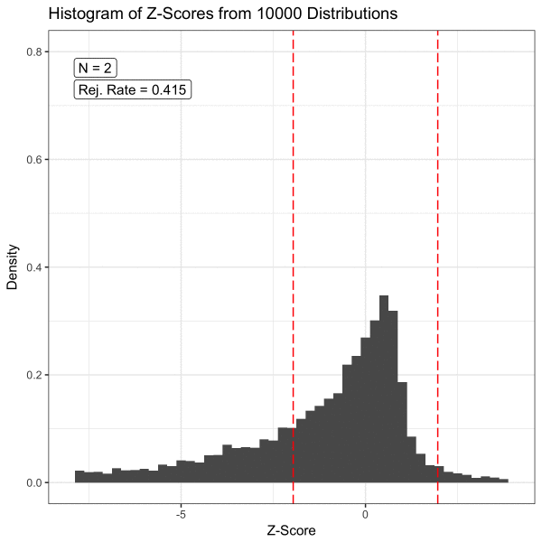
(Image from https://github.com/dfsnow/clt)